Why transform a Gaussian map at all?
Weak gravitational lensing measures how foreground matter distorts images of background galaxies. The convergence field, \(\kappa\), is a projected map of matter overdensity along the line of sight.
Correct two-point structure
A Gaussian random field can be generated to follow a specified power spectrum and cross-bin covariance.
No nonlinear tail
A Gaussian field does not naturally contain the asymmetric peaks, voids, skewness, or kurtosis created by nonlinear structure formation.
Add non-Gaussian structure
The GAN learns to turn the Gaussian ensemble into a generated ensemble that resembles cosmological simulations.
Here \(G\) is the generator, \(\kappa_{\mathrm{GRF}}\) is the Gaussian convergence input, and \(\widehat{\kappa}_{\mathrm{NG}}\) is the generated non-Gaussian candidate. The word candidate matters: the discriminator decides whether its local patches resemble real simulation patches.
From simulations to a tested generator
The project separates data construction, training, checkpoint selection, and held-out diagnostics so that validation and test maps do not leak into the training references.
flowchart TD
    A["Simulation files<br/>N × 4 × 256 × 256"]
    B["Select one bin or retain<br/>all four bins jointly"]
    C["Split complete simulation groups<br/>80% train · 10% validation · 10% test"]
    D["Estimate training-only Fourier covariance<br/>4 auto + 6 unique cross-spectra"]
    E["Synthesize independent correlated GRFs<br/>seed 42 · 25 radial covariance bins"]
    F["Normalize X and Y separately<br/>save μX, σX, μY, σY"]
    G["Generator U-Net<br/>GRF → generated NG candidate"]
    H["Real simulation candidate<br/>independent and unpaired"]
    I["Training-only physics references<br/>power + one-point moments"]
    J["PatchGAN discriminator<br/>local four-channel realism"]
    K["Generator objective<br/>adversarial + optional physics losses"]
    L["Validation every epoch<br/>no gradients or updates"]
    M["Save latest, periodic, and best checkpoints"]
    N["Held-out testing<br/>maps · PDF · ξ(r) · auto/cross-power"]

    A --> B --> C
    C --> D --> E --> F --> G
    C --> H
    C --> I
    G --> J
    H --> J
    J --> K
    I --> K
    K --> L --> M --> N

    classDef data fill:#ecfeff,stroke:#0891b2,color:#0f172a,stroke-width:2px;
    classDef model fill:#eef2ff,stroke:#4f46e5,color:#0f172a,stroke-width:2px;
    classDef loss fill:#fff1f2,stroke:#e11d48,color:#0f172a,stroke-width:2px;
    classDef result fill:#f0fdf4,stroke:#16a34a,color:#0f172a,stroke-width:2px;
    class A,B,C,D,E,F,H,I data;
    class G,J model;
    class K,L loss;
    class M,N result;
- Loading: read finite numeric NumPy arrays and preserve the channel order.
- Leakage-safe splitting: keep all bins from one simulation in exactly one split.
- GRF statistics: estimate input covariance only from training targets.
- Generation: create new independent GRF realizations with the desired covariance.
- Batching: deliver normalized tensors in batches of two.
- Adversarial learning: alternate discriminator and generator optimization.
- Physics constraints: compare generated ensemble statistics with fixed training references.
- Validation: measure generalization without updating either network.
- Checkpointing: save the best, latest stable, and periodic states.
- Testing: use the untouched 10% split for final maps and ensemble summaries.
Four views of the same cosmic structure
Every simulation file contains four convergence maps. Each channel corresponds to a source-redshift bin, so the bins observe related projected structure through different lensing kernels and path lengths.
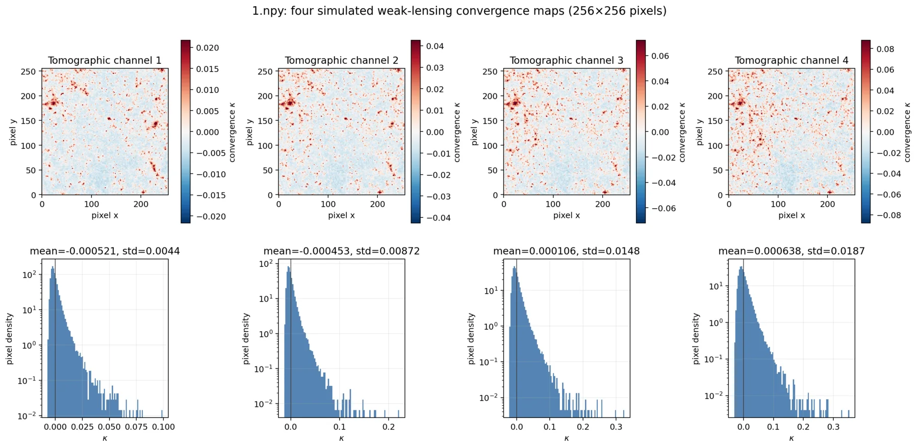
What the tensor shape means
Two independent model samples processed together in one optimizer step.
Four ordered tomographic redshift bins kept together as one sample.
256 pixel rows in the flat-sky convergence tile.
256 pixel columns in the same tile.
How 3,000 maps become 750 model samples
The command-line option --number-of-maps 3000
counts individual single-channel maps. Because every model sample uses
four channels, the main experiment loads \(3000/4=750\) simulation
groups. The deterministic group split gives:
| Split | Fraction | Four-channel samples | Purpose |
|---|---|---|---|
| Training | 80% | 600 | Update weights and build GRF/physics references |
| Validation | 10% | 75 | Select checkpoints and monitor generalization |
| Test | 10% | 75 | Final held-out ensemble diagnostics only |
Normalization
Neural networks train more stably when values are centered and similarly scaled. The loaded GRF ensemble \(X\) and target ensemble \(Y\) are standardized separately:
The four scalar constants \(\mu_X,\sigma_X,\mu_Y,\sigma_Y\) are saved in every checkpoint. For plots, the generated normalized map is converted back to physical convergence units with \(\widehat y=\sigma_Y\widehat y_{\mathrm{norm}}+\mu_Y\).
How the four redshift bins remain correlated
Four independent GRFs would destroy tomography. Instead, this pipeline estimates a complete scale-dependent \(4\times4\) Fourier covariance matrix and uses it to mix four white-noise fields.
\(i\) and \(j\) label tomographic bins; the tilde denotes a Fourier transform; the star denotes complex conjugation; and angle brackets mean an average over training realizations and Fourier modes in one radial bin.
flowchart TD
    A["600 training target groups<br/>validation/test excluded"]
    B["Subtract each map mean"]
    C["2D FFT of every channel"]
    D["Compute κ̃ᵢ κ̃ⱼ*<br/>for every bin pair i,j"]
    E["Radially average<br/>into 25 Fourier bins"]
    F["4 × 4 covariance C(k)<br/>at every radial scale"]
    G["Interpolate C(k)<br/>onto the 2D Fourier grid"]
    H["Symmetrize covariance"]
    I["Clip small negative eigenvalues<br/>from sampling noise"]
    J["Cholesky factorization<br/>C = LLᵀ"]
    K["Draw four independent<br/>white-noise fields z"]
    L["FFT white noise"]
    M["Mix channels<br/>κ̃G = Lz"]
    N["Set zero-frequency mode to zero"]
    O["Inverse FFT"]
    P["Four real correlated GRF channels<br/>matching auto/cross two-point statistics"]

    A --> B --> C --> D --> E --> F --> G --> H --> I --> J
    K --> L --> M
    J --> M --> N --> O --> P

    classDef data fill:#ecfeff,stroke:#0891b2,color:#0f172a,stroke-width:2px;
    classDef math fill:#f5f3ff,stroke:#7c3aed,color:#0f172a,stroke-width:2px;
    classDef result fill:#f0fdf4,stroke:#16a34a,color:#0f172a,stroke-width:2px;
    class A,B,C,D,E,K,L data;
    class F,G,H,I,J,M,N,O math;
    class P result;
Every building block used by the model
These definitions connect the code words to what physically happens to a \(256\times256\) convergence map.
- Tensor
- A multidimensional numerical array. A training batch is indexed by sample, channel, row, and column.
- Channel
- One ordered map plane. Here channels 1–4 represent four tomographic source-redshift bins.
- Feature map
- An internal learned representation. A feature channel might respond to peaks, edges, voids, or textures rather than a redshift bin.
- Convolution
- A small learned filter slides across the map and combines nearby pixels. The same filter weights are reused at every position.
- Kernel
- The local filter window. A 3×3 kernel reads a pixel and its eight immediate neighbours; a 4×4 kernel reads sixteen local values.
- Stride
- How far the kernel moves. Stride 1 checks every location; stride 2 moves two pixels and roughly halves the spatial resolution.
- Padding
- Extra boundary values supplied when a kernel reaches beyond an edge, allowing controlled output dimensions.
- Reflection padding
- Boundary values are mirrored from inside the map instead of inserting zeros. It reduces artificial dark borders but is not periodic padding.
- ReLU
- The activation \(\max(0,z)\). It keeps positive responses and sets negative responses to zero, making the network nonlinear.
- LeakyReLU
- Like ReLU, but negative values become \(0.2z\) rather than zero. This preserves a gradient for negative discriminator activations.
- Activation function
- A nonlinear transformation after a layer. Without it, many stacked convolutions would collapse into one linear operation.
- Max pooling
- A 2×2 window retains the largest response and advances by two pixels, reducing width and height while keeping strong local features.
- Encoder
- The contracting half of the U-Net. It reduces spatial resolution and increases feature channels to learn progressively broader context.
- Bottleneck
- The deepest 16×16, 512-channel representation. It has the widest contextual view but still retains a spatial grid.
- Decoder
- The expanding half of the U-Net. It restores the map resolution while combining deep context with saved fine-scale features.
- Bilinear upsampling
- A smooth interpolation that doubles height and width using nearby values, followed here by a learned convolution.
- Skip connection
- A direct path from an encoder scale to the matching decoder scale, preventing fine spatial information from being lost.
- Concatenation
- Stacking channels. A decoder feature tensor and its encoder skip tensor are joined along the channel axis.
- 1×1 convolution
- A learned channel mixer at each pixel. The final generator layer converts 32 features into four convergence outputs.
- Residual
- A learned correction added to an existing field. In physics mode the U-Net predicts what must be added to the GRF.
- Parameter
- A learned weight or bias. Optimization adjusts parameters to reduce the chosen loss.
- Batch
- A small group processed before one optimizer update. The project uses batch size 2 to fit 256² four-channel maps on available hardware.
- Epoch
- One complete pass through all 600 training samples. With batch size 2, one epoch contains 300 training batches.
- Loss function
- A differentiable numerical objective. Smaller is better for that specific term, but GAN losses must be interpreted jointly.
- Gradient
- The derivative of the loss with respect to each parameter; it indicates how a small parameter change alters the loss.
- Backpropagation
- Applying the chain rule backward through the computation graph to calculate all parameter gradients.
- Optimizer
- The rule that converts gradients into parameter updates. Both networks use Adam with \(\beta_1=0.5,\beta_2=0.999\).
- Learning rate
- The update scale. Too high can destabilize training; too low can make learning extremely slow.
- Logit
- An unrestricted discriminator score before sigmoid. Positive logits favour “real”; negative logits favour “generated.”
- BCE with logits
- Binary cross-entropy combined with sigmoid in one numerically stable operation.
- GroupNorm
- Normalizes groups of feature channels inside each sample, avoiding unreliable batch statistics when the batch size is only two.
- Fourier transform
- Rewrites a map as spatial-frequency modes. Large structures occupy low frequencies and fine structures occupy high frequencies.
- Power spectrum
- The average squared Fourier amplitude versus scale; a two-point statistical summary of spatial structure.
- One-point PDF
- The distribution of individual pixel values without using their locations. It exposes asymmetry, tails, peaks, skewness, and kurtosis.
- Two-point correlation
- The average product of map values separated by distance \(r\), measuring how pixels co-vary across spatial separation.
- Auto-power
- A spectrum within one bin, such as \(C_\ell^{11}\) or \(C_\ell^{44}\).
- Cross-power
- A spectrum between two bins, such as \(C_\ell^{41}=C_\ell^{14}\), measuring shared scale-dependent structure.
- Tomography
- Using multiple source-redshift slices to obtain depth-dependent information rather than one projected map alone.
The U-Net: compress context, then rebuild detail
The generator transforms a normalized four-channel GRF tensor into four generated channels. It contains 8,630,884 trainable parameters and no separate random-noise vector: with fixed weights, the same input produces the same output.
flowchart TB
    A["Correlated Gaussian input<br/>B × C × 256 × 256<br/>C = 1 or 4"]

    B["DoubleConv C → 32<br/>B × 32 × 256 × 256<br/>save x₁"]
    C["MaxPool + DoubleConv 32 → 64<br/>B × 64 × 128 × 128<br/>save x₂"]
    D["MaxPool + DoubleConv 64 → 128<br/>B × 128 × 64 × 64<br/>save x₃"]
    E["MaxPool + DoubleConv 128 → 256<br/>B × 256 × 32 × 32<br/>save x₄"]
    F["MaxPool + DoubleConv 256 → 512<br/>B × 512 × 16 × 16<br/>bottleneck"]

    G["Bilinear upsample + 3×3 Conv<br/>512 → 256 · 32 × 32"]
    H["Concatenate x₄<br/>DoubleConv 512 → 256"]
    I["Bilinear upsample + 3×3 Conv<br/>256 → 128 · 64 × 64"]
    J["Concatenate x₃<br/>DoubleConv 256 → 128"]
    K["Bilinear upsample + 3×3 Conv<br/>128 → 64 · 128 × 128"]
    L["Concatenate x₂<br/>DoubleConv 128 → 64"]
    M["Bilinear upsample + 3×3 Conv<br/>64 → 32 · 256 × 256"]
    N["Concatenate x₁<br/>DoubleConv 64 → 32"]

    O["Final 1×1 Conv<br/>32 → C"]
    P["Raw U-Net output r<br/>B × C × 256 × 256"]
    Q{"Selected loss mode"}
    R["Adversarial mode<br/>generated map = r"]
    S["Physics mode<br/>generated map = GRF in target units<br/>+ residual scale × r"]

    A --> B --> C --> D --> E --> F
    F --> G --> H --> I --> J --> K --> L --> M --> N --> O --> P --> Q
    E -. "skip x₄" .-> H
    D -. "skip x₃" .-> J
    C -. "skip x₂" .-> L
    B -. "skip x₁" .-> N
    Q --> R
    Q --> S

    classDef input fill:#ecfeff,stroke:#0891b2,color:#0f172a,stroke-width:2px;
    classDef encoder fill:#eff6ff,stroke:#2563eb,color:#0f172a,stroke-width:2px;
    classDef bottleneck fill:#fef3c7,stroke:#d97706,color:#0f172a,stroke-width:2px;
    classDef decoder fill:#f5f3ff,stroke:#7c3aed,color:#0f172a,stroke-width:2px;
    classDef output fill:#f0fdf4,stroke:#16a34a,color:#0f172a,stroke-width:2px;
    classDef choice fill:#fff1f2,stroke:#e11d48,color:#0f172a,stroke-width:2px;
    class A input;
    class B,C,D,E encoder;
    class F bottleneck;
    class G,H,I,J,K,L,M,N decoder;
    class O,P,R,S output;
    class Q choice;
Solid arrows show the main forward path. Dashed arrows are the four U-Net skip connections that move saved encoder features directly to the decoder at the same spatial resolution.
What happens inside one DoubleConv block?
flowchart LR
    A["Input feature tensor"]
    B["Reflection pad by 1 pixel"]
    C["3×3 convolution<br/>learn local features"]
    D["ReLU<br/>max(0,z)"]
    E["Reflection pad by 1 pixel"]
    F["3×3 convolution<br/>refine features"]
    G["ReLU<br/>max(0,z)"]
    H["Output<br/>same height and width"]
    A --> B --> C --> D --> E --> F --> G --> H
    classDef data fill:#ecfeff,stroke:#0891b2,color:#0f172a,stroke-width:2px;
    classDef conv fill:#eff6ff,stroke:#2563eb,color:#0f172a,stroke-width:2px;
    classDef activation fill:#fff7ed,stroke:#ea580c,color:#0f172a,stroke-width:2px;
    class A,H data;
    class B,C,E,F conv;
    class D,G activation;
Padding is one pixel on every side, so a stride-1 3×3 convolution
preserves height and width. Because padding mode is
reflect, pixels needed beyond the edge are mirrored from
inside the tile. For example, an edge sequence
[a, b, c, d] behaves locally like
[b, a, b, c, d, c] rather than being surrounded by zeros.
Layer-by-layer generator dimensions
| Stage | Operation | Output | Why it exists |
|---|---|---|---|
| Input | Normalized GRF | B × 4 × 256 × 256 | Four correlated tomographic fields |
| x₁ | DoubleConv 4→32 | B × 32 × 256 × 256 | Fine pixel-scale features |
| x₂ | Pool + DoubleConv 32→64 | B × 64 × 128 × 128 | Slightly broader spatial context |
| x₃ | Pool + DoubleConv 64→128 | B × 128 × 64 × 64 | Intermediate structures |
| x₄ | Pool + DoubleConv 128→256 | B × 256 × 32 × 32 | Coarse structures |
| Bottleneck | Pool + DoubleConv 256→512 | B × 512 × 16 × 16 | Deep multiscale context |
| Decoder 1 | Upsample, Conv, concat x₄, DoubleConv | B × 256 × 32 × 32 | Start spatial reconstruction |
| Decoder 2 | Upsample, Conv, concat x₃, DoubleConv | B × 128 × 64 × 64 | Combine context and intermediate detail |
| Decoder 3 | Upsample, Conv, concat x₂, DoubleConv | B × 64 × 128 × 128 | Restore smaller-scale structure |
| Decoder 4 | Upsample, Conv, concat x₁, DoubleConv | B × 32 × 256 × 256 | Recover full-resolution detail |
| Output | 1×1 Conv 32→4 | B × 4 × 256 × 256 | Produce one value per bin and pixel |
Where the 8,630,884 generator parameters are
| Generator component | Trainable parameters | Role |
|---|---|---|
| First encoder block, 4→32 | 10,432 | Convert four input bins into 32 learned features |
| Encoder down 1 | 55,424 | 32→64 features |
| Encoder down 2 | 221,440 | 64→128 features |
| Encoder down 3 | 885,248 | 128→256 features |
| Bottleneck block | 3,539,968 | 256→512 deepest representation |
| Decoder up 1 | 2,949,888 | 512 bottleneck to 256 decoded features |
| Decoder up 2 | 737,664 | 256→128 decoded features |
| Decoder up 3 | 184,512 | 128→64 decoded features |
| Decoder up 4 | 46,176 | 64→32 full-resolution features |
| Final 1×1 convolution | 132 | 32 features→4 output bins |
| Generator total | 8,630,884 | Approximately 92.5% of the complete GAN |
Direct output versus residual output
The U-Net output is the map
The network must learn both large-scale structure and non-Gaussian corrections through adversarial feedback alone.
The U-Net output is a correction
The GRF supplies the baseline field. The U-Net learns the residual needed to make it non-Gaussian; \(s=1\) in the main run.
A fresh physics run initializes the final convolution to zero. Therefore the initial residual is exactly zero and the complete initial output is the Gaussian input expressed in target-normalized units. Training then learns deviations from that controlled starting point.
A local realism critic with 900 overlapping decisions
The discriminator contains 695,649 parameters. It is unconditioned: it sees a real or generated four-channel candidate, but it never sees the corresponding Gaussian input.
flowchart TB
    A["Candidate convergence map<br/>real simulation or generated<br/>B × C × 256 × 256"]
    B["Reflection-padded Conv 4×4<br/>stride 2 · C → 32<br/>B × 32 × 128 × 128"]
    C["LeakyReLU<br/>negative slope = 0.2"]
    D["Reflection-padded Conv 4×4<br/>stride 2 · 32 → 64<br/>B × 64 × 64 × 64"]
    E["GroupNorm · 8 groups<br/>LeakyReLU 0.2"]
    F["Reflection-padded Conv 4×4<br/>stride 2 · 64 → 128<br/>B × 128 × 32 × 32"]
    G["GroupNorm · 8 groups<br/>LeakyReLU 0.2"]
    H["Reflection-padded Conv 4×4<br/>stride 1 · 128 → 256<br/>B × 256 × 31 × 31"]
    I["GroupNorm · 8 groups<br/>LeakyReLU 0.2"]
    J["Reflection-padded Conv 4×4<br/>stride 1 · 256 → 1"]
    K["B × 1 × 30 × 30 raw logits<br/>900 overlapping 70×70 patch judgments"]

    A --> B --> C --> D --> E --> F --> G --> H --> I --> J --> K

    classDef input fill:#ecfeff,stroke:#0891b2,color:#0f172a,stroke-width:2px;
    classDef conv fill:#eff6ff,stroke:#2563eb,color:#0f172a,stroke-width:2px;
    classDef norm fill:#f5f3ff,stroke:#7c3aed,color:#0f172a,stroke-width:2px;
    classDef output fill:#fff1f2,stroke:#e11d48,color:#0f172a,stroke-width:2px;
    class A input;
    class B,D,F,H,J conv;
    class C,E,G,I norm;
    class K output;
Why is it called PatchGAN?
The final output is not one global “real/fake” number. It is a 30×30 grid, giving 900 logits for each map. One logit depends on a 70×70 input region. Neighbouring logits have centers separated by eight pixels, so their judged regions overlap strongly.
| Layer | Receptive field | Patch-center spacing | Interpretation |
|---|---|---|---|
| Conv 1 | 4×4 | 2 pixels | Very local texture |
| Conv 2 | 10×10 | 4 pixels | Small structures |
| Conv 3 | 22×22 | 8 pixels | Intermediate structures |
| Conv 4 | 46×46 | 8 pixels | Broader patch context |
| Conv 5 | 70×70 | 8 pixels | Final local realism judgment |
Avoids inserting zero-valued borders near patch edges.
Normalizes within each sample, making it stable for batch size two.
The network returns logits; BCEWithLogitsLoss handles sigmoid internally.
Where the 695,649 discriminator parameters are
| Discriminator component | Trainable parameters | Notes |
|---|---|---|
| Conv 1, 4→32 | 2,080 | First four-channel local filters |
| Conv 2, 32→64 | 32,832 | Second stride-2 convolution |
| GroupNorm 64 | 128 | One scale and shift per channel |
| Conv 3, 64→128 | 131,200 | Third stride-2 convolution |
| GroupNorm 128 | 256 | One scale and shift per channel |
| Conv 4, 128→256 | 524,544 | Stride-1 patch refinement |
| GroupNorm 256 | 512 | One scale and shift per channel |
| Conv 5, 256→1 | 4,097 | Produces the 30×30 logit grid |
| Discriminator total | 695,649 | Approximately 7.5% of the complete GAN |
Two networks learn through different gradient paths
The generated tensor is used twice: detached when teaching the discriminator, and connected to the computation graph when teaching the generator.
flowchart TB
    X["Gaussian input x"] --> GEN["Generate complete map ŷ = G(x)"]
    Y["Independent real simulation y"]

    subgraph DUP["A · Discriminator update — scheduled every 2 generator steps"]
        Y --> NR["Add current instance noise<br/>real candidate"]
        GEN --> DET["Detach generated tensor<br/>stop gradient into G"]
        DET --> NF["Add the same instance noise<br/>fake candidate"]
        NR --> DR["D(real) → 30×30 logits"]
        NF --> DF["D(fake) → 30×30 logits"]
        DR --> LR["BCE real target = 0.9"]
        DF --> LF["BCE fake target = 0"]
        LR --> LD["LD = Lreal + Lfake"]
        LF --> LD
        LD --> BD["Backpropagate and update D only"]
    end

    subgraph GUP["B · Generator update — every batch"]
        GEN --> LIVE["Use generated tensor without detach"]
        LIVE --> FREEZE["Freeze discriminator parameters"]
        FREEZE --> DG["D(ŷ) → generated patch logits"]
        DG --> ADV["Generator adversarial BCE<br/>target = 1"]
        LIVE --> LOW["Low-frequency preservation loss"]
        LIVE --> POW["Radial power-spectrum loss"]
        LIVE --> ONE["One-point moment loss"]
        ADV --> TOTAL["Total generator objective"]
        LOW --> TOTAL
        POW --> TOTAL
        ONE --> TOTAL
        TOTAL --> BG["Backpropagate through frozen D<br/>and update G only"]
        BG --> ENABLE["Re-enable discriminator gradients"]
    end

    classDef source fill:#ecfeff,stroke:#0891b2,color:#0f172a,stroke-width:2px;
    classDef operation fill:#eff6ff,stroke:#2563eb,color:#0f172a,stroke-width:2px;
    classDef loss fill:#fff1f2,stroke:#e11d48,color:#0f172a,stroke-width:2px;
    classDef update fill:#f0fdf4,stroke:#16a34a,color:#0f172a,stroke-width:2px;
    class X,Y source;
    class GEN,NR,DET,NF,DR,DF,LIVE,FREEZE,DG,ENABLE operation;
    class LR,LF,LD,ADV,LOW,POW,ONE,TOTAL loss;
    class BD,BG update;
Discriminator objective
Label smoothing changes the real target from 1.0 to 0.9. The fake target stays 0. The code sums the real and fake losses; it does not divide their sum by two.
Generator adversarial objective
The generator tries to move every fake patch logit toward the “real” target. Discriminator parameters are frozen for this update, but its operations remain differentiable, so gradients continue backward into the generator.
Physics-mode generator objective
| Term | Weight | What is compared | Why it is needed |
|---|---|---|---|
| Adversarial BCE | 1 | Generated patch logits against real target 1 | Local non-Gaussian realism |
| Low-frequency L1 | 10 | Generated and input Fourier modes below 0.125 Nyquist | Preserve large-scale GRF structure |
| Radial power | 5 | Log generated ensemble-mean power against fixed training power in 20 bins | Control spatial variance versus scale |
| One-point statistics | 1 | Mean, standard deviation, skewness, and excess kurtosis | Control the asymmetric pixel distribution and tails |
Main physics-run hyperparameters
2 × 10⁻⁴
Adam step scale for the U-Net.
1 × 10⁻⁵
Lower rate to prevent D from racing ahead.
Every 2 G steps
Generator still updates every batch.
0.1 → 0
Linearly decays over the first 20 epochs.
- Set deterministic Python, NumPy, and PyTorch seeds.
- Select CUDA if available, otherwise Apple MPS, otherwise CPU.
- Construct the four-channel U-Net and four-channel PatchGAN.
- For a fresh physics run, zero-initialize the generator output layer.
- Build fixed power and moment references from training targets only.
- Loop over 300 training batches per epoch.
- Update the discriminator on its scheduled batches.
- Update the generator on every batch.
- Average each metric over the number of samples, not just batches.
- Run 38 validation batches with both networks in evaluation mode.
- Save history, quick validation maps, and checkpoint states.
Automatic collapse monitoring
GAN loss is a competition, so a very strong discriminator can starve the
generator of useful gradients. The configured safety check can stop when
either discriminator train/validation loss falls below 0.4 while either
generator adversarial train/validation loss exceeds 2.0, after the warm-up.
The rejected state is saved separately as collapse_detected.pt.
What is saved, where it goes, and which state to use
Every checkpoint stores the epoch, both networks, both Adam optimizer states, complete metric history, command-line arguments, normalization constants, and number of channels.
best.pt
Use for the main validation/test result because physics mode selects it using the lowest validation total generator loss.
latest.pt
Use to continue from the most recent accepted stable epoch with matching run settings.
epoch_XXXX.pt
Use when comparing the same held-out test input across exact saved epochs.
Reproducible training command
python train_original.py \
  --tomographic-bin all \
  --number-of-maps 3000 \
  --grf-radial-bins 25 \
  --loss-function physics \
  --epochs 500 \
  --run-tag physics_joint_3000maps_v1
On resume, --epochs 500 means continue until the total
epoch number reaches 500; it does not add 500 more epochs.
Reading the maps and statistics together
These figures were generated from the physics run's epoch-219 checkpoint. Ensemble spectra use all 75 held-out test realizations. The checkpoint is a captured training state, not a claim that epoch 219 is the final or best scientific model.
The 6×6 diagnostic layout
| Column | Quantity | Question answered |
|---|---|---|
| 1 | Correlated Gaussian input | What field entered the four-channel generator? |
| 2 | Real simulation, unpaired | What does one independent target-distribution sample look like? |
| 3 | Generated map | What non-Gaussian candidate did the generator produce? |
| 4 | One-point PDF | Does the generated pixel distribution reproduce the simulation peak and tails? |
| 5 | Two-point correlation | Does generated spatial correlation versus pixel separation resemble the simulation? |
| 6 | Fourier input-output correlation | At which scales does the generated output preserve the GRF input? |
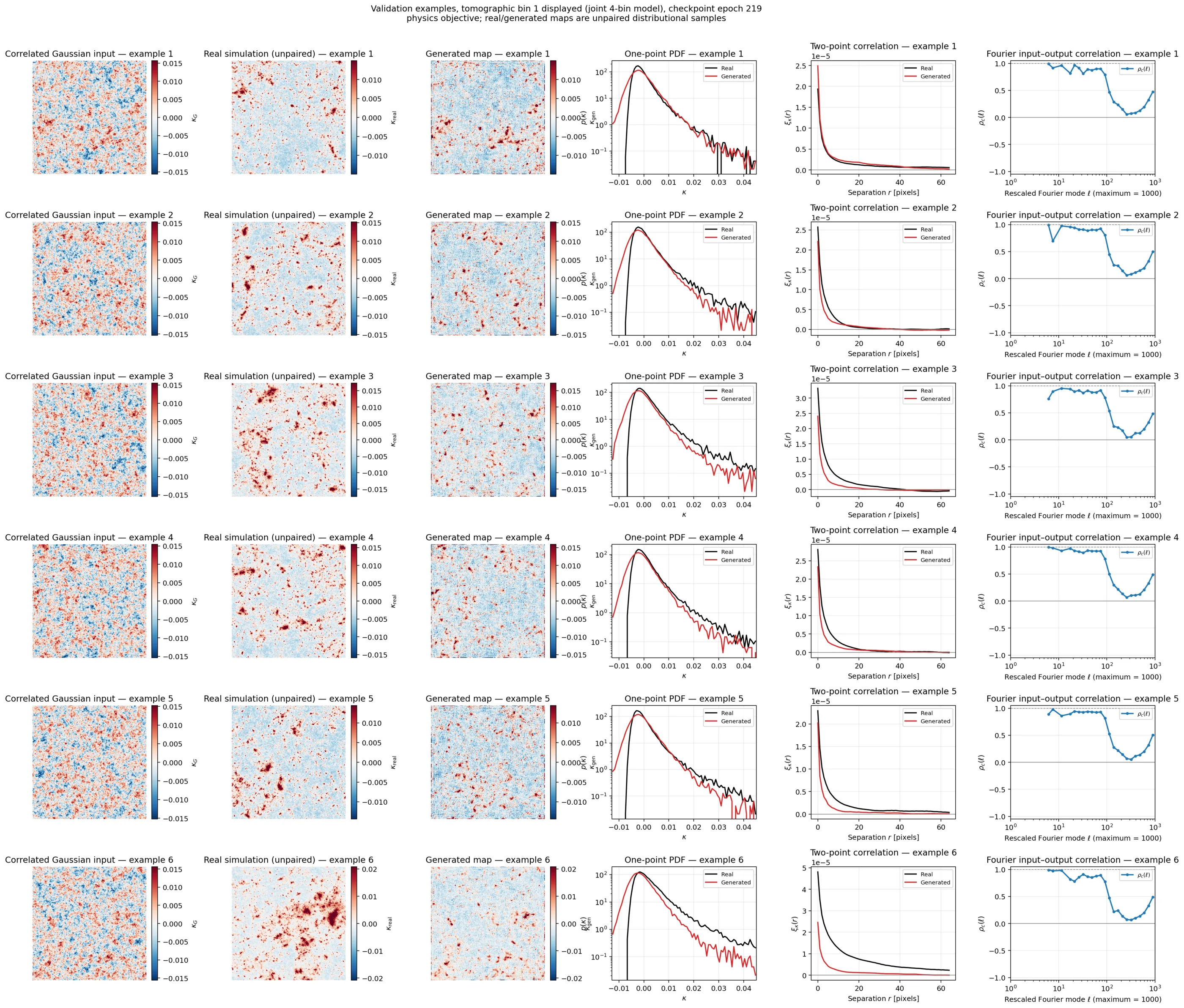
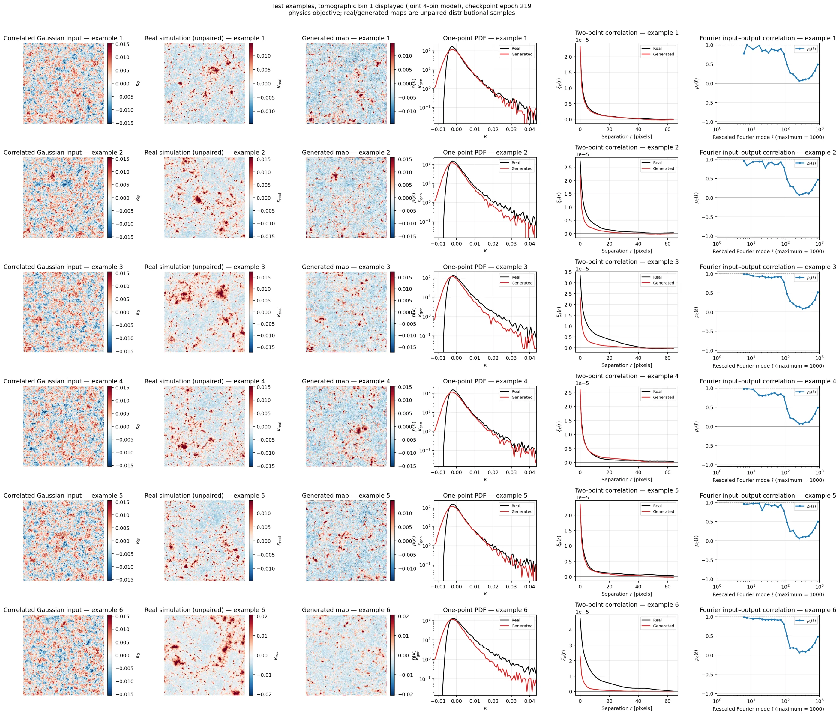
Training history
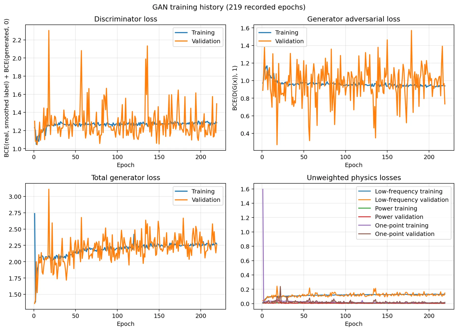
GAN losses need not decrease monotonically because each network is learning against a moving opponent. The validation curves fluctuate more strongly because only 75 validation samples are available. A useful interpretation combines stability of the curves with visual and statistical diagnostics.
Held-out bin-1 power spectrum
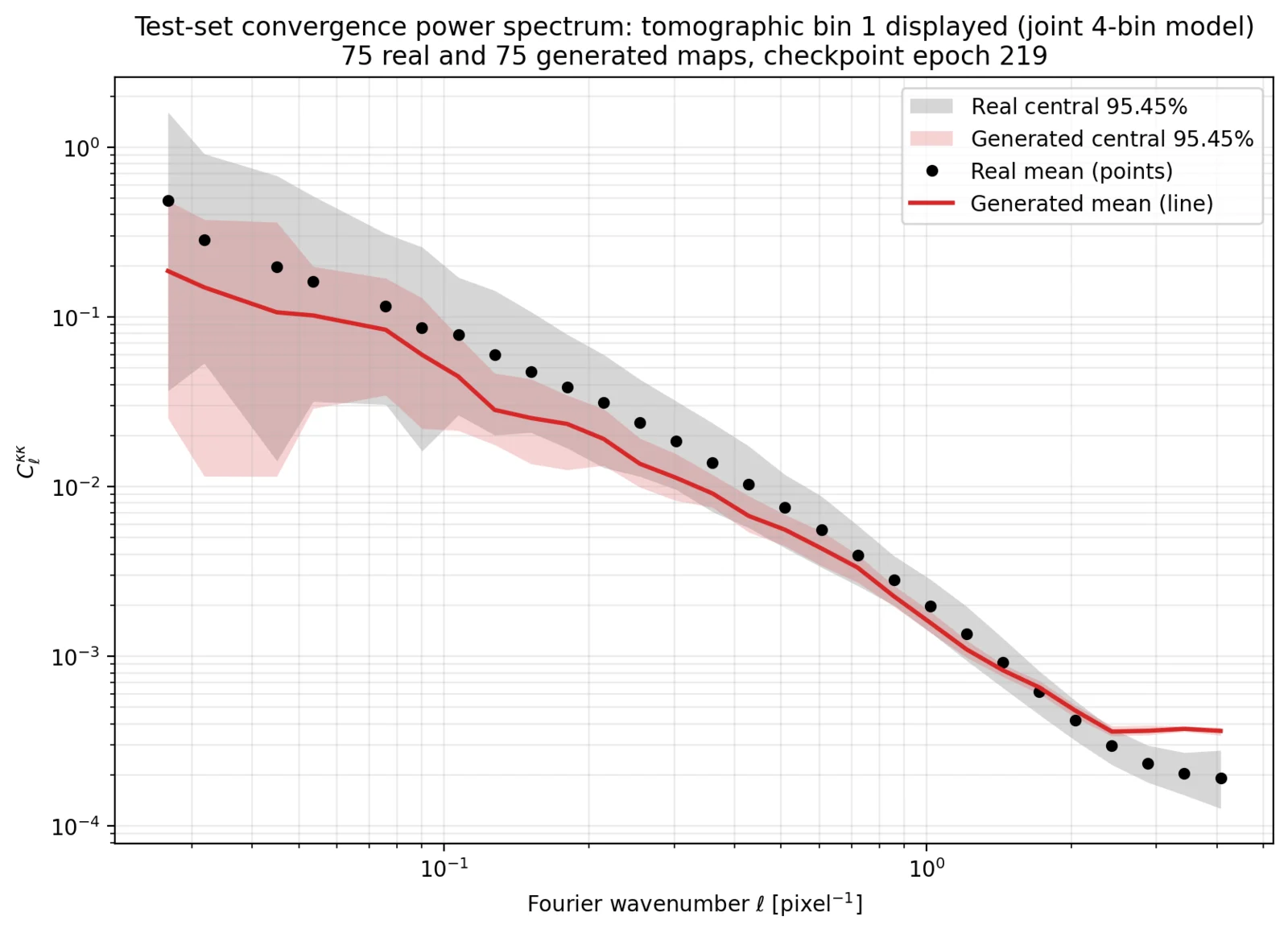
At low Fourier wavenumber, the generated mean is below the simulation mean in this checkpoint. The curves become closer over intermediate and high modes, with a small generated high-mode floor near the right edge. This diagnostic therefore identifies scale-dependent agreement and disagreement that a visually realistic map alone cannot reveal.
Tomographic auto- and cross-power
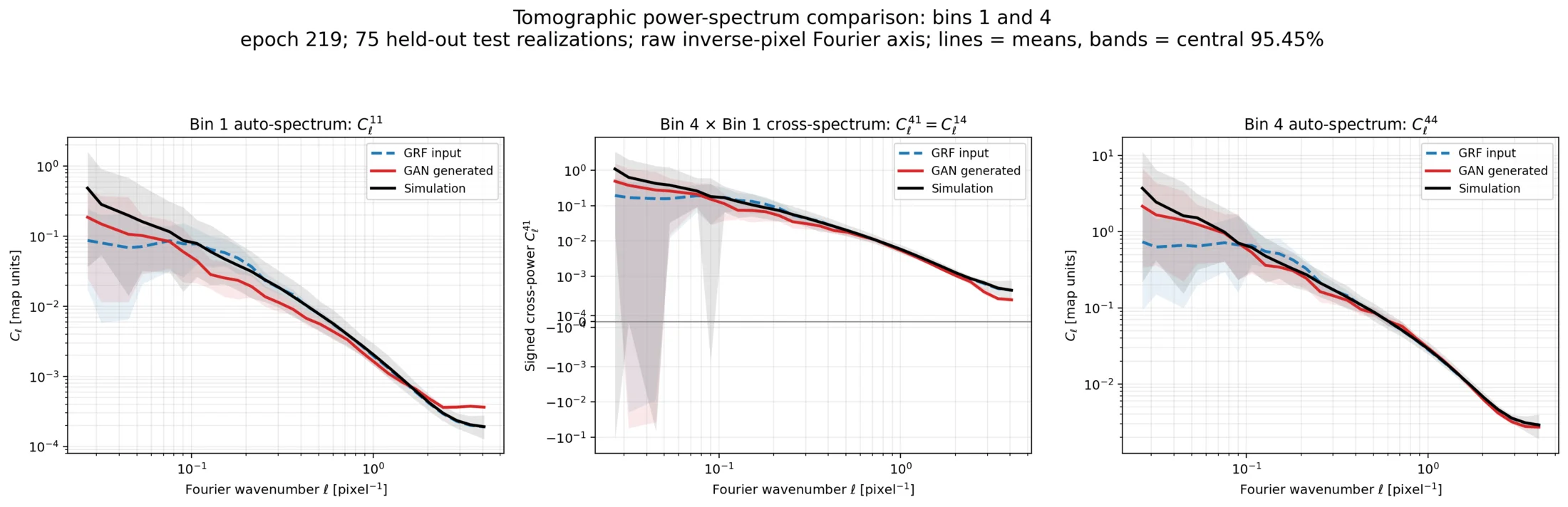
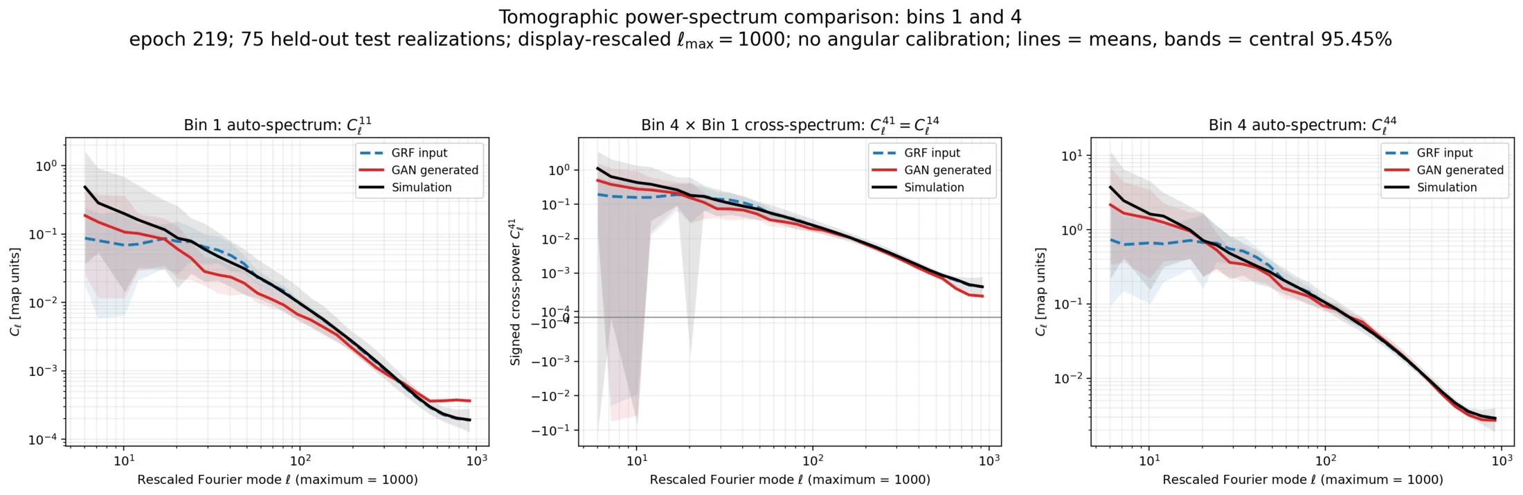
Bin-1 auto-spectrum
Tests spatial structure within the lowest displayed tomographic bin.
Bin-4/bin-1 cross-spectrum
Tests whether the generated endpoint bins retain the correct shared structure.
Bin-4 auto-spectrum
Tests spatial structure within the highest displayed tomographic bin.
Where the trained generator enters a shear pipeline
The trained network can be treated as a deterministic transformation with frozen parameters. The conceptual replacement is to generate the non-Gaussian convergence field before converting convergence into shear.
flowchart TD
    A["KGRF<br/>four correlated Gaussian<br/>convergence channels"]
    B["Convert external array<br/>to B × 4 × 256 × 256"]
    C["Normalize using μX and σX<br/>stored in checkpoint"]
    D["Frozen generator in eval mode<br/>no parameter changes"]
    E["U-Net raw correction r"]
    F["Physics output rule<br/>x in target units + residual scale × r"]
    G["Denormalize using μY and σY"]
    H["Kgen<br/>generated non-Gaussian convergence"]
    I["Kaiser–Squires transform<br/>γ₁, γ₂ = KZshear(Kgen)"]
    J["Likelihood / MCMC / Monte Carlo inference"]

    A --> B --> C --> D --> E --> F --> G --> H --> I --> J

    classDef source fill:#ecfeff,stroke:#0891b2,color:#0f172a,stroke-width:2px;
    classDef bridge fill:#eff6ff,stroke:#2563eb,color:#0f172a,stroke-width:2px;
    classDef model fill:#f5f3ff,stroke:#7c3aed,color:#0f172a,stroke-width:2px;
    classDef result fill:#f0fdf4,stroke:#16a34a,color:#0f172a,stroke-width:2px;
    class A source;
    class B,C,G bridge;
    class D,E,F model;
    class H,I,J result;
def KGRF_to_Kgen(k_grf, generator, normalization):
    # 1. Convert the external array to PyTorch shape (B, 4, 256, 256)
    # 2. Normalize using the constants stored in the checkpoint
    # 3. Run the frozen generator with gradients disabled
    # 4. Apply the physics residual rule used during training
    # 5. Convert back to physical convergence units
    # 6. Return in the array format expected by the inference code
    return k_gen

k_gen = KGRF_to_Kgen(k_grf, generator, normalization)
gamma1, gamma2 = KZshear(k_gen)
Important interface requirements
- Load the exact selected checkpoint and set the generator to evaluation mode.
- Freeze its parameters; inference should not retrain the network.
- Keep all four tomographic channels in their training order.
- Use the checkpoint's saved normalization rather than recomputing it.
- Apply the same direct or physics residual output rule used during training.
- Convert between JAX and PyTorch arrays without silently changing axis order or precision.
- Decide whether gradients through the generator are required by the inference sampler.
- Validate the wrapper independently using shapes, moments, spectra, and deterministic repeatability.
What the present model establishes—and what remains
Scientific limitations
- Unpaired supervision: the model learns ensemble similarity, not a unique simulation counterpart for each GRF.
- Unconditioned discriminator: local realism does not guarantee preservation of a specific input realization.
- No cosmological conditioning: cosmological parameters are not explicit network inputs.
- No source metadata in the arrays: exact redshift edges, cosmology, angular scale, and noise assumptions must be documented separately.
- Reflection boundaries: the convolution convention is not periodic and may affect patches near an edge.
- Display versus physical \(\ell\): angular calibration is required before interpreting spectra as cosmological multipoles.
- GAN loss ambiguity: neither a small D loss nor a small G adversarial loss is sufficient evidence of scientific fidelity.
- Inference validation remains essential: parameter posteriors must be checked for bias after inserting the generator into the lensing likelihood or sampler.
Next validation targets
All ten unique tomographic spectra
Compare four auto-spectra and all six cross-spectra, not only the bin-1/bin-4 endpoint subset.
Higher-order statistics
Add peak counts, Minkowski functionals, bispectrum summaries, and scale-dependent moments.
Boundary and calibration checks
Test periodic convolutions and obtain the physical angular pixel scale for true \(\ell\) axes.
Inference closure tests
Run synthetic truth-recovery experiments and verify unbiased posteriors before scientific deployment.
Reproducibility record
A scientific result should record the Git commit, checkpoint and stored epoch, number of maps, split seed, GRF seed, radial covariance bins, loss weights, both learning rates, device and library versions, tomographic channel order, and angular pixel size used for any physical spectrum.